Data

The main dataset for our project is a combined dataset from summary datasets made by United Nations Development Program, World Bank, Kaggle, and World Health Organization. It can be access at here. This dataset has a range from 1985 to 2016. However, since there is very few data in 2016, we will only keep the range from 1985 to 2015.

The raw dataset has a size of 27660 observations and 8 features. Basic features we are interested in include:

Country
Year: Year of the records
Sex
Age: Age groups including “5-14”, “15-24”, “25-34”, “35-54”, “55-74”, and “75+”.
GDP per capita
Suicides_no: Amount of suicides

Besides those, we will derive our main interested variable, Suicides Per 100K as Suicides_no divided by Population and multiplied by 100,000.

Exploratory data analysis

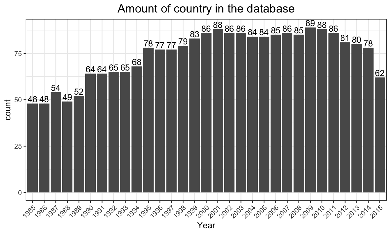
Country

There are on average, 74.3548387 countries in the dataset across each year. Graph below shows the distribution. Although there are less countries before 1995, the amount of countries for each year is stable around 80.

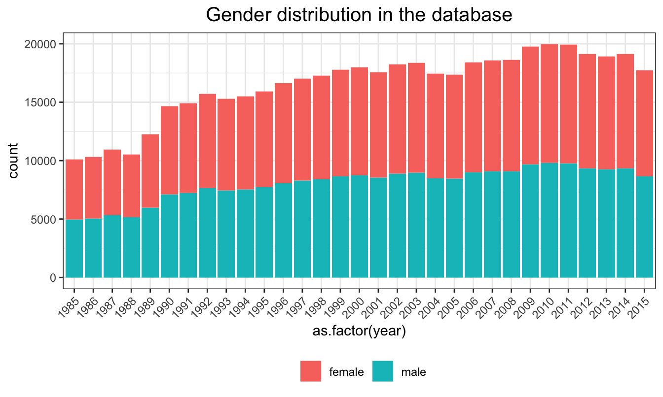
Sex

The graph below shows that sex for each year is also evenly distributed.

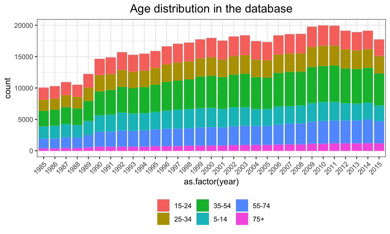
Age group

Although there are some variations between groups, the ratios between amounts of people in different age groups are consistent across years.

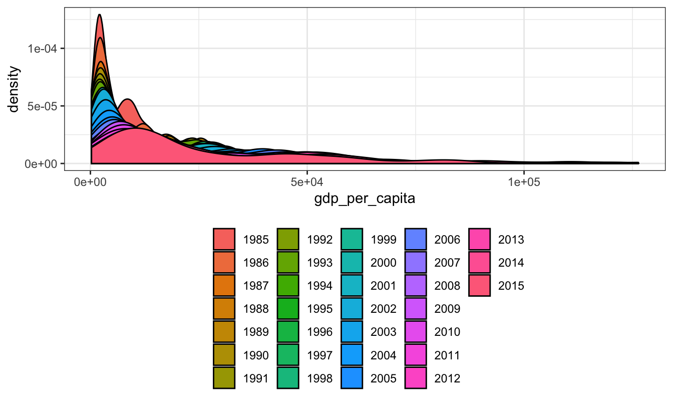
GDP per capita

The distribution of GDP per capita is skewed to the right. As the year goes on, we can see that the distribution becomes flatter, relatively.

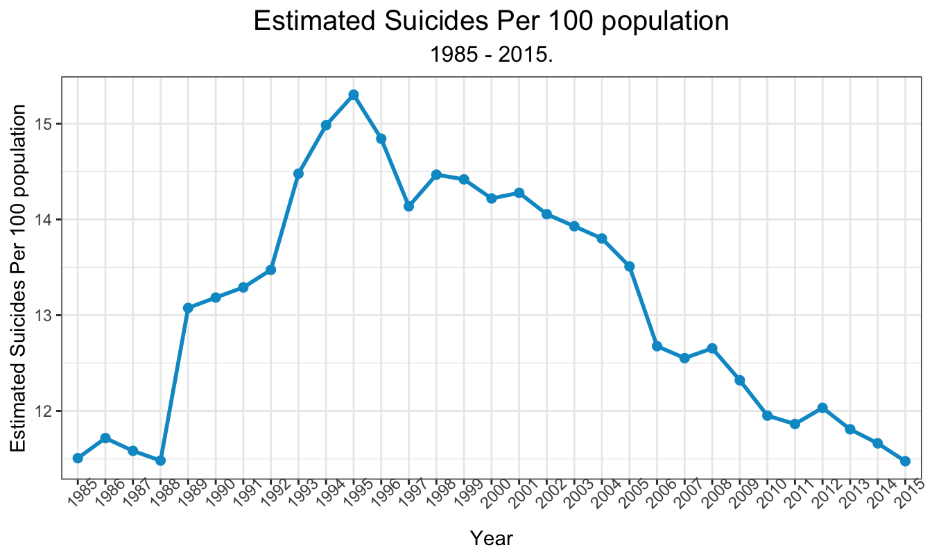
Suicides Per 100K

As we mentioned above, we can derive our main interested variable, Suicides Per 100K, as Suicides_no divided by Population and multiplied by 100,000. The trend is shown as below. As we can see, in recent years, the estimated suicides rates are decreasing.

Statistical Analysis

Visualization will be used to examine the global general trend. We will detect the group difference by sex, age, and GDP per capita by doing regression analysis. The interaction terms between age group and sex are also considered since it’s possible that sex can have different suicide trend regarding to different age groups. For example, women in menopause might have higher suicide rate because of the hormonal fluctuation. Lastly, although it is out of our primary interest, we will fit a regression model to see whether there is a sign of national-specific trend.

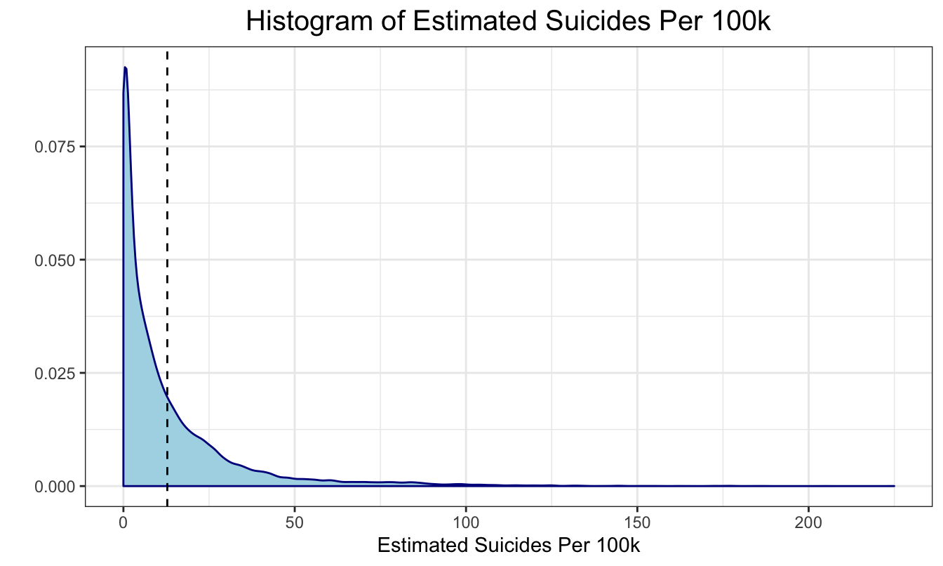
Following is the distribution of suicide_100k_pop, we can see that we need to transform it to satisfy the assumptions of the linear model.

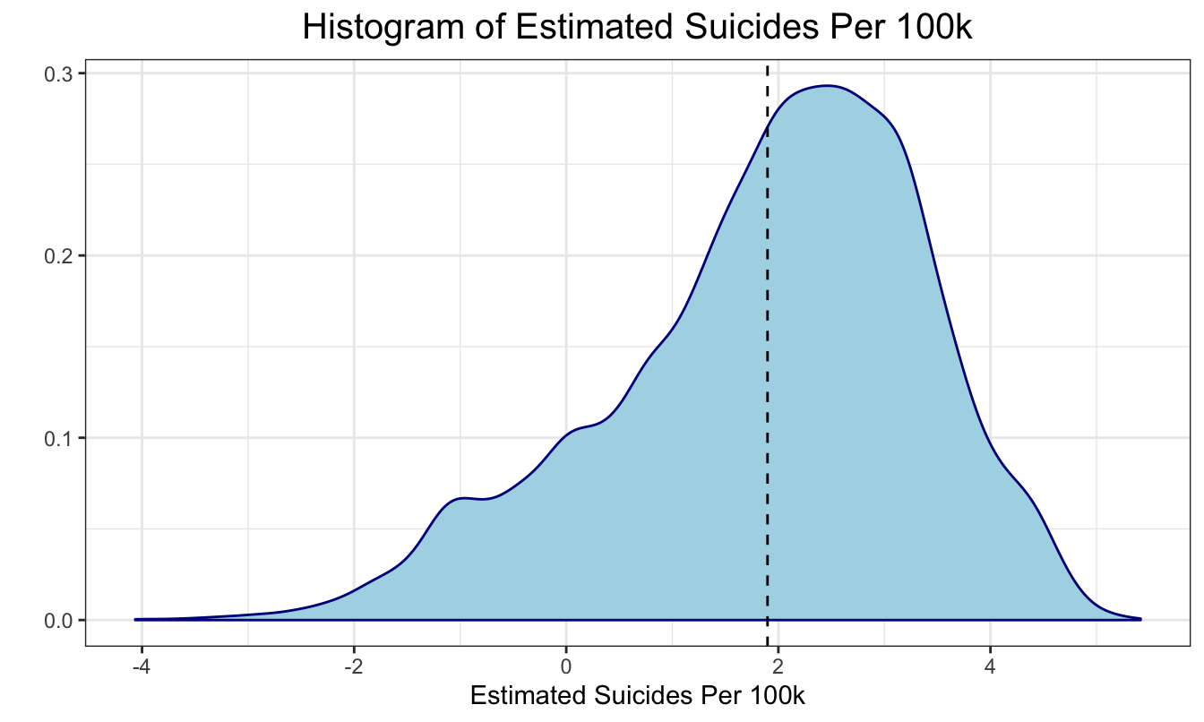
We used log transformation and changed 0’s to 0.01 for further calculations. Following graphs show that after the transformation, the distribution had been much more normal than the previous one.

Results

Based on transformation above, the model we are going to fit is:

\[ log(suicide \space per \space 100k) = \beta_0 + \beta_1year + \beta_2sex + \beta_3 age + \beta_4 age*sex + \beta_5 gdp \space per \space capita\]

	Estimate	Std. Error	t value	Pr(>\|t\|)
(Intercept)	20.4128030	1.6138338	12.648641	0.0000000
year	-0.0096925	0.0008074	-12.004703	0.0000000
sexmale	1.0971519	0.0313288	35.020566	0.0000000
age25-34	0.0827020	0.0313288	2.639807	0.0083000
age35-54	0.2699173	0.0313288	8.615630	0.0000000
age5-14	-1.6251063	0.0313288	-51.872616	0.0000000
age55-74	0.3531358	0.0313288	11.271926	0.0000000
age75+	0.4404010	0.0313288	14.057388	0.0000000
gdp_per_capita	0.0000067	0.0000004	18.529951	0.0000000
sexmale:age25-34	0.2767489	0.0443056	6.246365	0.0000000
sexmale:age35-54	0.2562206	0.0443056	5.783030	0.0000000
sexmale:age5-14	-0.8449252	0.0443056	-19.070394	0.0000000
sexmale:age55-74	0.1647189	0.0443056	3.717790	0.0002014
sexmale:age75+	0.2615484	0.0443056	5.903282	0.0000000

Based on the summary, we can see that all our main effects and the interaction term are statistically significant. This indicates that there indeed are group differences by age, gender, and GDP per capita. As we proposed, sex can have different suicide trends regarding to different age groups.

The F-statistics is 2221.3144029. It’s obvious that the model is statistically significant under any reasonable critical value. It also has a \(R^2\) value of 0.5108901, which indicated chosen variables together are able to explain \(51.09\%\) of observed variation.

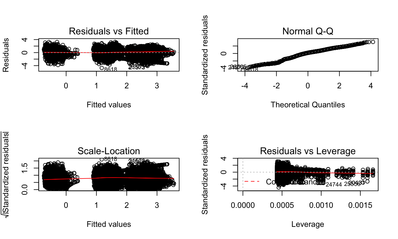
To ensure accuracy, we also examined the assumptions of our model. The Residuals vs Fitted and Scale-Location value plot show that the model is nearly homostaticity. Normality assumption is examined by the Q-Q plot, which is satisfied. Lastly, the Residuals vs Leverage plot indicates that although there are about 3 potential outliers in our dataset, none of them is close enough to the contour of cook’s distance to be considered as influential observations.

In addition, we fitted another model by adding country and population into previous model.

\[ log(suicide \space per \space 100k) = \beta_0 + \beta_1year + \beta_2sex + \beta_3 age + \beta_4 age*sex + \beta_5 gdp \space per \space capita + \beta_6 Country\]

The anova result indicates that at least one of the countries and population variable is statistically significant. This means that a more micro studies such as national level suicide trend analysis can be a topic for future research questions.

## Analysis of Variance Table
## 
## Model 1: log_suicide ~ country + sex + age + gdp_per_capita + sex * age
## Model 2: log_suicide ~ year + sex * age + gdp_per_capita
##   Res.Df   RSS  Df Sum of Sq      F    Pr(>F)    
## 1  27548 16220                                   
## 2  27646 31272 -98    -15052 260.86 < 2.2e-16 ***
## ---
## Signif. codes:  0 '***' 0.001 '**' 0.01 '*' 0.05 '.' 0.1 ' ' 1

Conclusion

Our regression model indicates that all our main effects (i.e. age_group, sex, GDP per capita) and the interaction term between age_group and sex are statistically significant. This indicates that there indeed are group difference by age and gender. As we proposed, gender can have different impacts on amount of suicides regarding to different age groups. An interesting finding is that although there is no obvious trend between amount of suicides and GDP per capita based on the graph, the regression output shows that GDP per capita does have a statistically significant effect on amount of suicides.

Discussion

A strength of this study is that the study is a longitudinal study with a time spin of 30 years, which gives us more chance to explore the justifications and the trends behind the data. Meanwhile, there are many limitations that future researchers need to be aware of. First of all, there are only few variables that may be related to suicide rate. However, there are other factors or latent factors that may be reflected by suicide rate such as alcoholic use. Secondly, since we had done a global trend analysis, we need data from all over the world. However, this particular data set is lack of the suicide information from Asia(especially China and North Korea) and Africa. Lastly, the data is not individual-leveled which may intervene with our analysis for prediction purposes.

Regression Analysis